Every linear transformation $T:\mathbb{R}^n \to \mathbb{R}^m$ can be represented as a matrix product with a matrix $M_T \in \mathbb{R}^{m \times n}$. Suppose that the transformation $T$ is defined in a word description like “Let $T$ be the counterclockwise rotation of all points in the $xy$-plane by $30^\circ$.” How do we find the matrix $M_T$ that corresponds to this transformation?

In this section we will discuss various useful linear transformations and derive their matrix representations. The goal of this section is to solidify the bridge in your understanding between the abstract specification of a transformation $T(\vec{v})$ and its specific implementation of this transformation as a matrix-vector product $M_T\vec{v}$.

Once you find the matrix representation of a given transformation you can “apply” that transformation to many vectors. For example, if you know the $(x,y)$ coordinates of each pixel of an image, and you replace these coordinates with the outcome of the matrix-vector product $M_T(x,y)^T$, you'll obtain a rotated version of the image. That is essentially what happens when you use the “rotate” tool inside an image editing program.

In the previous section we learned about linear transformations and their matrix representations:

• $T:\mathbb{R}^{n} \to \mathbb{R}^{m}$:

A linear transformation, which takes inputs $\vec{v} \in \mathbb{R}^{n}$ and produces outputs vector $\vec{w} \in \mathbb{R}^{n}$: $T(\vec{v}) = \vec{w}$.

• $M_T \in \mathbb{R}^{m\times n}$:

A matrix representation of the linear transformation $T$.

The action of the linear transformation $T$ is equivalent to a multiplication by the matrix $M_T$: \[ \vec{w} = T(\vec{v}) \qquad \Leftrightarrow \qquad \vec{w} = M_T \vec{v}. \]

In order to find the matrix representation of the transformation $T \colon \mathbb{R}^n \to \mathbb{R}^m$ it is sufficient to “probe” $T$ with the $n$ vectors from the standard basis for the input space $\mathbb{R}^n$: \[ \hat{e}_1 \equiv \begin{bmatrix} 1 \nl 0 \nl \vdots \nl 0 \end{bmatrix} \!\!, \ \ \ \hat{e}_2 \equiv \begin{bmatrix} 0 \nl 1 \nl \vdots \nl 0 \end{bmatrix}\!\!, \ \ \ \ \ldots, \ \ \ \hat{e}_n \equiv \begin{bmatrix} 0 \nl \vdots \nl 0 \nl 1 \end{bmatrix}\!\!. \] The matrix $M_T$ which corresponds to the action of $T$ on the standard basis is \[ M_T = \begin{bmatrix} | & | & \mathbf{ } & | \nl T(\vec{e}_1) & T(\vec{e}_2) & \dots & T(\vec{e}_n) \nl | & | & \mathbf{ } & | \end{bmatrix}. \]

This is an $m\times n$ matrix that has as its columns the outputs of $T$ for the $n$ probes.

The first kind of linear transformation we will study is the projection.

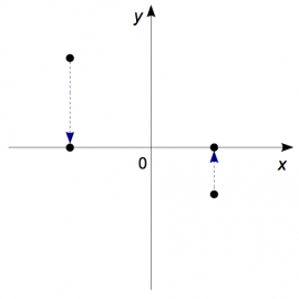Consider the projection onto the $x$-axis $\Pi_{x}$. The action of $\Pi_x$ on any vector or point is to leave the $x$-coordinate unchanged and set the $y$-coordinate to zero.

We can find the matrix associated with this projection by analyzing how it transforms the two vectors of the standard basis: \[ \begin{bmatrix} 1 \nl 0 \end{bmatrix} = \Pi_x\!\!\left( \begin{bmatrix} 1 \nl 0 \end{bmatrix} \right), \qquad \begin{bmatrix} 0 \nl 0 \end{bmatrix} = \Pi_x\!\!\left( \begin{bmatrix} 0 \nl 1 \end{bmatrix} \right). \] The matrix representation of $\Pi_x$ is therefore given by: \[ M_{\Pi_{x}}= \begin{bmatrix} \Pi_x\!\!\left( \begin{bmatrix} 1 \nl 0 \end{bmatrix} \right) & \Pi_x\!\!\left( \begin{bmatrix} 0 \nl 1 \end{bmatrix} \right) \end{bmatrix} = \left[\begin{array}{cc} 1 & 0 \nl 0 & 0 \end{array}\right]. \]

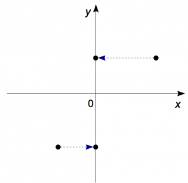Can you guess what the matrix for the projection onto the $y$-axis will look like? We use the standard approach to compute the matrix representation of $\Pi_y$: \[ M_{\Pi_{y}}= \begin{bmatrix} \Pi_y\!\!\left( \begin{bmatrix} 1 \nl 0 \end{bmatrix} \right) & \Pi_y\!\!\left( \begin{bmatrix} 0 \nl 1 \end{bmatrix} \right) \end{bmatrix} = \left[\begin{array}{cc} 0 & 0 \nl 0 & 1 \end{array}\right]. \]

We can easily verify that the matrices $M_{\Pi_{x}}$ and $M_{\Pi_{y}}$ do indeed select the appropriate coordinate from a general input vector $\vec{v} = (v_x,v_y)^T$: \[ \begin{bmatrix} 1 & 0 \nl 0 & 0 \end{bmatrix} \begin{bmatrix} v_x \nl v_y \end{bmatrix} = \begin{bmatrix} v_x \nl 0 \end{bmatrix}, \qquad \begin{bmatrix} 0 & 0 \nl 0 & 1 \end{bmatrix} \begin{bmatrix} v_x \nl v_y \end{bmatrix} = \begin{bmatrix} 0 \nl v_y \end{bmatrix}. \]

Recall that the general formula for the projection of a vector $\vec{v}$ onto another vector $\vec{a}$ is obtained as follows: \[ \Pi_{\vec{a}}(\vec{v})=\left(\frac{\vec{a} \cdot \vec{v} }{ \| \vec{a} \|^2 }\right)\vec{a}. \]

Thus, if we wanted to compute the projection onto an arbitrary direction $\vec{a}$, we would have to compute: \[ M_{\Pi_{\vec{a}}}= \begin{bmatrix} \Pi_{\vec{a}}\!\!\left( \begin{bmatrix} 1 \nl 0 \end{bmatrix} \right) & \Pi_{\vec{a}}\!\!\left( \begin{bmatrix} 0 \nl 1 \end{bmatrix} \right) \end{bmatrix}. \]

We can also compute the projection of the vector $\vec{v} \in \mathbb{R}^3$ onto some plane $P: \ \vec{n}\cdot\vec{x}=n_xx+n_yy+n_zz=0$ as follows: \[ \Pi_{P}(\vec{v}) = \vec{v} - \Pi_{\vec{n}}(\vec{v}). \] The interpretation of the above formula is as follows. We compute the part of the vector $\vec{v}$ that is in the $\vec{n}$ direction, and then we subtract this part from $\vec{v}$ to obtain a point in the plane $P$.

To obtain the matrix representation of $\Pi_{P}$ we calculate what it does to the standard basis $\hat{\imath}=\hat{e}_1 = (1,0,0)^T$, $\hat{\jmath}=\hat{e}_2 = (0,1,0)^T$ and $\hat{k} =\hat{e}_3 = (0,0,1)^T$.

We can obtain a projection matrix onto any unit vector as an outer product of the vector with itself. Let us consider as an example how we could find the matrix for the projection onto the $x$-axis $\Pi_x(\vec{v}) = (\hat{\imath}\cdot \vec{v})\hat{\imath}=M_{\Pi_x}\vec{v}$. Recall that the inner product (dot product) between two column vectors $\vec{u}$ and $\vec{v}$ is equivalent to the matrix product $\vec{u}^T \vec{v}$, while their outer product is given by the matrix product $\vec{u}\vec{v}^T$. The inner product corresponds to a $1\times n$ matrix times a $n \times 1$ matrix, so the answer is $1 \times 1$ matrix, which is equivalent to a number: the value of the dot product. The outer product corresponds to $n\times 1$ matrix times a $1 \times n$ matrix so the answer is an $n \times n$ matrix. For example the projection matrix onto the $x$-axis is given by the matrix $M_{\Pi_x} = \hat{\imath}\hat{\imath}^T$.

What? Where did that equation come from? To derive this equation you simply have to rewrite the projection formula in terms of the matrix product and use the commutative law of scalar multiplication $\alpha \vec{v} = \vec{v}\alpha$ and the associative law of matrix multiplication $A(BC)=(AB)C$. Check it: \[ \begin{align*} \Pi_x(\vec{v}) = (\hat{\imath}\cdot\vec{v})\:\hat{\imath} = \hat{\imath} (\hat{\imath}\cdot\vec{v}) & = \hat{\imath} (\hat{\imath}^T \vec{v} ) = \left[\begin{array}{c} 1 \nl 0 \end{array}\right] \left( \left[\begin{array}{ccc} 1 & 0 \end{array}\right] \left[\begin{array}{c} v_x \nl v_y \end{array}\right] \right) \nl & = \left(\hat{\imath} \hat{\imath}^T\right) \vec{v} = \left( \left[\begin{array}{c} 1 \nl 0 \end{array}\right] \left[\begin{array}{ccc} 1 & 0 \end{array}\right] \right) \left[\begin{array}{c} v_x \nl v_y \end{array}\right] \nl & = \left(M \right) \vec{v} = \begin{bmatrix} 1 & 0 \nl 0 & 0 \end{bmatrix} \left[\begin{array}{c} v_x \nl v_y \end{array}\right] = \left[\begin{array}{c} v_x \nl 0 \end{array}\right]. \end{align*} \] We see that outer product $M\equiv\hat{\imath}\hat{\imath}^T$ corresponds to the projection matrix $M_{\Pi_x}$ which we were looking for.

More generally, the projection matrix onto a line with direction vector $\vec{a}$ is obtained by constructing a the unit vector $\hat{a}$ and then calculating the outer product: \[ \hat{a} \equiv \frac{ \vec{a} }{ \| \vec{a} \| }, \qquad M_{\Pi_{\vec{a}}}=\hat{a}\hat{a}^T. \]

Find the projection matrix $M_d \in \mathbb{R}^{2 \times 2 }$ for the projection $\Pi_d$ onto the $45^\circ$ diagonal line, a.k.a. “the line with equation $y=x$”.

The line $y=x$ corresponds to the parametric equation $\{ (x,y) \in \mathbb{R}^2 | (x,y)=(0,0) + t(1,1), t\in \mathbb{R}\}$, so the direction vector is $\vec{a}=(1,1)$. We need to find the matrix which corresponds to $\Pi_d(\vec{v})=\left( \frac{(1,1) \cdot \vec{v} }{ 2 }\right)(1,1)^T$.

The projection matrix onto $\vec{a}=(1,1)$ is computed most easily using the outer product approach. First we compute a normalized direction vector $\hat{a}=(\tfrac{1}{\sqrt{2}},\tfrac{1}{\sqrt{2}})$ and then we compute the matrix product: \[ M_d = \hat{a}\hat{a}^T = \begin{bmatrix} \tfrac{1}{\sqrt{2}} \nl \tfrac{1}{\sqrt{2}} \end{bmatrix} \begin{bmatrix} \tfrac{1}{\sqrt{2}} & \tfrac{1}{\sqrt{2}} \end{bmatrix} = \begin{bmatrix} \frac{1}{2} & \frac{1}{2} \nl \frac{1}{2} & \frac{1}{2} \end{bmatrix}. \]

Note that the notion of an outer product is usually not covered in a first linear algebra class, so don't worry about outer products showing up on the exam. I just wanted to introduce you to this equivalence between projections onto $\hat{a}$ and the outer product $\hat{a}\hat{a}^T$, because it is one of the fundamental ideas of quantum mechanics.

The “probing with the standard basis approach” is the one you want to remember for the exam. We can verify that it gives the same answer: \[ M_{d}= \begin{bmatrix} \Pi_d\!\!\left( \begin{bmatrix} 1 \nl 0 \end{bmatrix} \right) & \Pi_d\!\!\left( \begin{bmatrix} 0 \nl 1 \end{bmatrix} \right) \end{bmatrix} = \begin{bmatrix} \left(\frac{\vec{a} \cdot \hat{\imath} }{ \| \vec{a} \|^2 }\right)\!\vec{a} & \left(\frac{\vec{a} \cdot \hat{\jmath} }{ \| \vec{a} \|^2 }\right)\!\vec{a} \end{bmatrix} = \begin{bmatrix} \frac{1}{2} & \frac{1}{2} \nl \frac{1}{2} & \frac{1}{2} \end{bmatrix}. \]

Any projection matrix $M_{\Pi}$ satisfies $M_{\Pi}M_{\Pi}=M_{\Pi}$. This is one of the defining properties of projections, and the technical term for this is idempotence: the operation can be applied multiple times without changing the result beyond the initial application.

Note that a projection acts very differently on different sets of input vectors. Some input vectors are left unchanged and some input vectors are killed. Murder! Well, murder in a mathematical sense, which means being multiplied by zero.

Let $\Pi_S$ be the projection onto the space $S$, and $S^\perp$ be the orthogonal space to $S$ defined by $S^\perp = \{ \vec{w} \in \mathbb{R}^n \ | \ \vec{w} \cdot S = 0\}$. The action of $\Pi_S$ is completely different on the vectors from $S$ and $S^\perp$. All vectors $\vec{v} \in S$ comes out unchanged: \[ \Pi_S(\vec{v}) = \vec{v}, \] whereas vectors $\vec{w} \in S^\perp$ will be killed \[ \Pi_S(\vec{w}) = 0\vec{w} = \vec{0}. \] The action of $\Pi_S$ on any vector from $S^\perp$ is equivalent a multiplication by zero. This is why we call $S^\perp$ the null space of $M_{\Pi_S}$.

We can easily compute the matrices for simple reflections in the standard two-dimensional space $\mathbb{R}^2$.

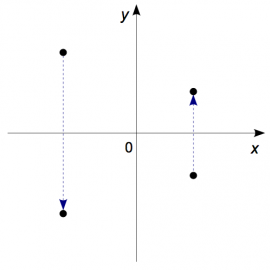The reflection through the $x$-axis should leave the $x$-coordinate unchanged and flip the sign of the $y$-coordinate.

We obtain the matrix by probing as usual: \[ M_{R_x}= \begin{bmatrix} R_x\!\!\left( \begin{bmatrix} 1 \nl 0 \end{bmatrix} \right) & R_x\!\!\left( \begin{bmatrix} 0 \nl 1 \end{bmatrix} \right) \end{bmatrix} = \begin{bmatrix} 1 & 0 \nl 0 & -1 \end{bmatrix}. \]

Which correctly sends $(x,y)^T$ to $(x,-y)^T$ as required.

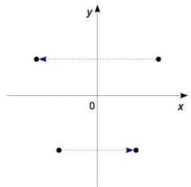The matrix associated with $R_y$, the reflection through the $y$-axis is given by: \[ M_{R_y}= \left[\begin{array}{cc} -1 & 0 \nl 0 & 1 \end{array}\right]. \] The numbers in the above matrix tell you to change the sign of the $x$-coordinate and leave the $y$-coordinate unchanged. In other words, everything that was to the left of the $y$-axis, now has to go to the right and vice versa.

Do you see how easy and powerful this matrix formalism is? You simply have to put in each column whatever you want the happen to the $\hat{e}_1$ vector and in the second column whatever you want to happen to the $\hat{e}_2$ vector.

Suppose we want to find the formula for the reflection through the line $y=x$, which passes right through the middle of the first quadrant. We will call this reflection $R_{d}$ (this time, my dear reader the diagram is on you to draw). In words though, what we can say is that $R_d$ makes $x$ and $y$ “swap places”.

Starting from the description “$x$ and $y$ swap places” it is not difficult to see what the matrix should be: \[ M_{R_d}= \left[\begin{array}{cc} 0 & 1 \nl 1 & 0 \end{array}\right]. \]

I want to point out that an important property that all reflection have. We can always identify the action of a reflection by the fact that it does two very different things to two sets of points: (1) some points are left unchanged by the reflection and (2) some points become the exact negatives of themselves.

For example, the points that are invariant under $R_{y}$ are the points that lie on the $y$-axis, i.e., the multiples of $(0,1)^T$. The points that become the exact negative of themselves are those that only have an $x$-component, i.e, the multiples of $(1,0)^T$. The acton of $R_y$ on all other points can be obtained as a linear combination of the “leave unchanged” and the “multiply by $-1$” actions. We will discuss this line of reasoning more at the end of this section and we will sey generally how to describe the actions of $R_y$ on its different input subspaces.

What about reflections through an arbitrary line? Consider the line $\ell: \{ \vec{0} + t\vec{a}, t\in\mathbb{R}\}$ that passes through the origin. We can write down a formula for the reflection through $\ell$ in terms of the projection formula: \[ R_{\vec{a}}(\vec{v})=2\Pi_{\vec{a}}(\vec{v})-\vec{v}. \] The reasoning behind the this formula is as follows. First we compute the projection of $\vec{v}$ onto the line $\Pi_{\vec{a}}(\vec{v})$, then take two steps in that direction and subtract $\vec{v}$ once. Use a pencil to annotate the figure to convince yourself the formula works.

Similarly, we can also derive and expression for the reflection through an arbitrary plane $P: \ \vec{n}\cdot\vec{x}=0$: \[ R_{P}(\vec{v}) =2\Pi_{P}(\vec{v})-\vec{v} =\vec{v}-2\Pi_{\vec{n}}(\vec{v}). \]

The first form of the formula uses a reasoning similar to the formula for the reflection through a line.

The second form of the formula can be understood as computing the shortest vector from the plane to $\vec{v}$, subtracting that vector once from $\vec{v}$ to get to a point in the plane, and subtracting it a second time to move to the point $R_{P}(\vec{v})$ on the other side of the plane.

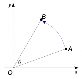We now want to find the matrix which corresponds to the counterclockwise rotation by the angle $\theta$. An input point $A$ in the plane will get rotated around the origin by an angle $\theta$ to obtain a new point $B$.

By now you know the drill. Probe with the standard basis: \[ M_{R_\theta}= \begin{bmatrix} R_\theta\!\!\left( \begin{bmatrix} 1 \nl 0 \end{bmatrix} \right) & R_\theta\!\!\left( \begin{bmatrix} 0 \nl 1 \end{bmatrix} \right) \end{bmatrix}. \] To compute the values in the first column, observe that the point $(1,0)=1\angle 0=(1\cos0,1\sin0)$ will be moved to the point $1\angle \theta=(\cos \theta, \sin\theta)$. The second input $\hat{e}_2=(0,1)$ will get rotated to $(-\sin\theta,\cos \theta)$. We therefore get the matrix: \[ M_{R_\theta} = \begin{bmatrix} \cos\theta &-\sin\theta \nl \sin\theta &\cos\theta \end{bmatrix}. \]

Finding the matrix representation of a linear transformation is like a colouring-book activity for mathematicians—you just have to fill in the columns.

Can you tell me what the inverse matrix of $M_{R_\theta}$ is?

You could use the formula for finding the inverse of a $2 \times 2$ matrix or you could use the $[ \: A \: |\; I \;]$-and-RREF algorithm for finding the inverse, but both of these approaches would be waaaaay too much work for nothing. I want you to try to guess the formula intuitively. If $R_\theta$ rotates stuff by $+\theta$ degrees, what do you think the inverse operation will be?

Yep! You got it. The inverse operation is $R_{-\theta}$ which rotates stuff by $-\theta$ degrees and corresponds to the matrix \[ M_{R_{-\theta}} = \begin{bmatrix} \cos\theta &\sin\theta \nl -\sin\theta &\cos\theta \end{bmatrix}. \] For any vector $\vec{v}\in \mathbb{R}^2$ we have $R_{-\theta}\left(R_{\theta}(\vec{v})\right)=\vec{v}=R_{\theta}\left(R_{-\theta}(\vec{v})\right)$ or in terms of matrices: \[ M_{R_{-\theta}}M_{R_{\theta}} = I = M_{R_{\theta}}M_{R_{-\theta}}. \] Cool no? That is what representation really means, the abstract notion of composition of linear transformations is represented by the matrix product.

What is the inverse operation to the reflection through the $x$-axis $R_x$? Reflect again!

What is the inverse matrix for some projection $\Pi_S$? Good luck finding that one. The whole point of projections is to send some part of the input vectors to zero (the orthogonal part) so a projection is inherently many to one and therefore not invertible. You can also see this from its matrix representation: if a matrix does not have full rank then it is not invertible.

At this point I am sure that you feel confident to face any linear transformation $T:\mathbb{R}^2\to\mathbb{R}^2$ and find its matrix $M_T \in \mathbb{R}^{2\times 2}$ by probing with the standard basis. But what if you are not allowed to probe $T$ with the standard basis? What if you are given the outputs of $T$ for some other basis $\{ \vec{v}_1, \vec{v}_2 \}$: \[ \begin{bmatrix} t_{1x} \nl t_{1y} \end{bmatrix} = T\!\!\left( \begin{bmatrix} v_{1x} \nl v_{1y} \end{bmatrix} \right), \qquad \begin{bmatrix} t_{2x} \nl t_{2y} \end{bmatrix} = T\!\!\left( \begin{bmatrix} v_{2x} \nl v_{2y} \end{bmatrix} \right). \] Can we find the matrix for $M_T$ given this data?

Yes we can. Because the vectors form a basis, we can reconstruct the information about the matrix $M_T$ from the input-output data provided. We are looking for four unknowns $m_{11}$, $m_{12}$, $m_{21}$, and $m_{22}$ that make up the matrix $M_T$: \[ M_T = \begin{bmatrix} m_{11} & m_{12} \nl m_{21} & m_{22} \end{bmatrix}. \] Luckily, the input-output data allows us to write four equations: \[ \begin{align} m_{11}v_{1x} + m_{12} v_{1y} & = t_{1x}, \nl m_{21}v_{1x} + m_{22} v_{1y} & = t_{1y}, \nl m_{11}v_{2x} + m_{12} v_{2y} & = t_{2x}, \nl m_{21}v_{2x} + m_{22} v_{2y} & = t_{2y}. \end{align} \] We can solve this system of equations using the usual techniques and find the coefficients $m_{11}$, $m_{12}$, $m_{21}$, and $m_{22}$.

Let's see how to do this in more detail. We can think of the entries of $M_T$ as a $4\times 1$ vector of unknowns $\vec{x}=(m_{11}, m_{12}, m_{21}, m_{22})^T$ and then rewrite the four equations as a matrix equation: \[ A\vec{x} = \vec{b} \qquad \Leftrightarrow \qquad \begin{bmatrix} v_{1x} & v_{1y} & 0 & 0 \nl 0 & 0 & v_{1x} & v_{1y} \nl v_{2x} & v_{2y} & 0 & 0 \nl 0 & 0 & v_{2x} & v_{2y} \end{bmatrix} \begin{bmatrix} m_{11} \nl m_{12} \nl m_{21} \nl m_{22} \end{bmatrix} = \begin{bmatrix} t_{1x} \nl t_{1y} \nl t_{2x} \nl t_{2y} \end{bmatrix}. \] We can then solve for $\vec{x}$ by finding $\vec{x}=A^{-1}\vec{b}$. As you can see, it is a little more work than probing with the standard basis, but it is still doable.

Probing the transformation $T$ with any basis should give us sufficient information to determine its matrix with respect to the standard basis using the above procedure. Given the freedom we have for choosing the “probing basis”, is there a natural basis for probing each transformation $T$? The standard basis is good for computing the matrix representation, but perhaps there is another choice of basis which would make the abstract description of $T$ simpler.

Indeed, this is the case. For many linear transformations there exists a basis $\{ \vec{e}_1, \vec{e}_2, \ldots \}$ such that the action of $T$ on the basis vector $\vec{e}_i$ is equivalent to the scaling of $\vec{e}_i$ by a constant $\lambda_i$: \[ T(\vec{e}_i) = \lambda_i \vec{e}_i. \]

Recall for example how projections leave some vectors unchanged (multiply by $1$) and send some vectors to zero (multiply by $0$). These subspaces of the input space are specific to each transformation and are called the eigenspaces (own spaces) of the transformation $T$.

As another example, consider the reflection $R_x$ which has two eigenspaces.

1. The space of vectors that are left unchanged

(the eigenspace correspondence to $\lambda=1$),

  which is spanned by the vector $(1,0)$:
  \[
    R_x\!\!\left(    \begin{bmatrix} 1 \nl 0 \end{bmatrix} \right)
    = 1 \begin{bmatrix} 1 \nl 0 \end{bmatrix}.
  \]
- The space of vectors which become the exact negatives of themselves
  (the eigenspace correspondence to $\lambda=-1$), 
  which is spanned by $(0,1)$:
  \[
    R_x\!\!\left(    \begin{bmatrix} 0 \nl 1 \end{bmatrix} \right)
    = -1 \begin{bmatrix} 0 \nl 1 \end{bmatrix}.
  \]

From the theoretical point of view, describing the action of $T$ in its natural basis is the best way to understand what it does. For each of the eigenvectors in the various eigenspaces of $T$, the action of $T$ is a simple scalar multiplication!

In the next section we will study the notions of eigenvalues and eigenvectors in more detail. Note, however, that you are already familiar with the special case of the “zero eigenspace”, which we call the null space. The action of $T$ on the vectors in its null space is equivalent to a multiplication by the scalar $0$.