We defined the integral operation $\int f(x)\;dx$ as the inverse operation of $\frac{d}{dx}$, but it is important to know how to think of the integral operation on its own. No course on calculus would be complete without a telling of the classical “rectangles story” of integral calculus.

• $x$: $\in \mathbb{R}$, the argument of the function.
• $f(x)$: a function $f \colon \mathbb{R} \to \mathbb{R}$.
• $x_i$: where the sum starts, i.e., some given point on the $x$ axis.
• $x_f$: where the sum stops.
• $A(x_i,x_f)$: Exact value of the area under the curve $f(x)$ from $x=x_i$ to $x=x_f$.
• $S_n(x_i,x_f)$: An approximation to the area $A$ in terms of

$n$ rectangles.

• $s_k$: Area of $k$-th rectangle when counting from the left.

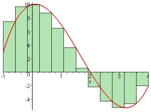
In the picture on the right, we are approximating the function $f(x)=x^3-5x^2+x+10$ between $x_i=-1$ and $x_f=4$ using $n=12$ rectangles. The sum of the areas of the 12 rectangles is what we call $S_{12}(-1,4)$. We say that $S_{12}(-1,4) \approx A(-1,4)$.

The main formula you need to know is that the combined area approximation is given by the sum of the areas of the little rectangles: $$S_n = \sum_{k=1}^{n} s_k.$$

Each of the little rectangles has an area $s_k$ given by its height multiplied by its width. The height of each rectangle will vary, but the width is constant. Why constant? Riemann figured that having each rectangle with a constant width $\Delta x$ would make it very easy to calculate the approximation. The total length of the interval from $x_i$ to $x_f$ is $(x_f-x_i)$. If we divide this length into $n$ equally spaced segments, each of width $\Delta x$ given by: $$\Delta x = \frac{x_f - x_i}{n}.$$

OK, we have the formula for the width figured out, let's see what the height will be for the $k$-th rectangle, where $k$ is our counter from left to right in the sequence of rectangles. The height of the function varies as we move along the $x$ axis. For the rectangles, we pick isolated “samples” of $f(x)$ for the following values $$x_k = x_i + k\Delta x, \textrm{ for } k \in \{ 1, 2, 3, \ldots, n \},$$ all of them equally spaced $\Delta x$ apart.

The area of each rectangle is height times width: $$s_k = f(x_i + k\Delta x)\Delta x.$$

Now, my dear students, I want you to stare at the above equation and do some simple calculations to check that you understand. There is no point in continuing if you are just taking my word for it. Verify that when $k=1$, the formula gives the area of the first little rectangle. Verify also that when $k=n$, the formula for the $x_n$ gives the right value ($x_f$).

Ok let's put our formula for $s_k$ in the sum where it belongs. The Riemann sum approximation using $n$ rectangles is given by $$S_n = \sum_{k=1}^{n} f(x_i + k\Delta x)\Delta x,$$ where $\Delta x =\frac{|x_f - x_i|}{n}$.

Let us get back to the picture where we try to approximate the area under the curve $f(x)=x^3-5x^2+x+10$ by using 12 pieces.

For this scenario the value we would get for the 12-rectangle approximation to the area under the curve with $$S_{12} = \sum_{k=1}^{12} f(x_i + k\Delta x)\Delta x = 11.802662.$$ You shouldn't trust me though, but always check for yourself using live.sympy.org by typing in the following expressions:

 >>> n=12.0; xk = -1 + k*5/n; sk = (xk**3-5*xk**2+xk+10)*(5/n);
 >>> summation( sk, (k,1,n) )
      11.802662...

Who cares though? This is such a crappy approximation! You can clearly see that some rectangles lie outside of the curve (overestimates), and some are too far inside (underestimates). You might be wondering why I wasted so much of your time to achieve such a lousy approximation. We have not been wasting our time. You see, the Riemann sum formula $S_n$ gets better and better as you cut the region into smaller and smaller rectangles.

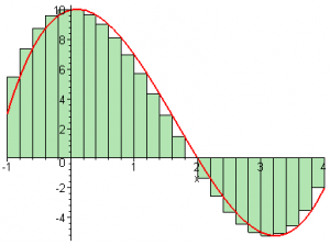
With $n=25$, we get a more fine grained approximation in which the sum of the rectangles is given by: $$S_{25} = \sum_{k=1}^{25} f(x_i + k\Delta x)\Delta x = 12.4.$$

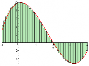
Then for $n=50$ we get: $$S_{50} = 12.6625.$$

For $n=100$ the sum of the rectangles areas is starting to look pretttttty much like the function. The calculation gives us $S_{100} = 12.790625$.

For $n=1000$ we get $S_{1000} = 12.9041562$ which is very close to the actual value of the area under the curve: $$A(-1,4) = 12.91666\ldots$$

You see in the long run, when $n$ gets really large the rectangle approximation (Riemann sum) can be made arbitrarily good. Imagine you cut the region into $n=10000$ rectangles, wouldn't $S_{10000}(-1,4)$ be a pretty accurate approximation of the actual area $A(-1,4)$?

The fact that you can approximate the area under the curve with a bunch of rectangles is what integral calculus is all about. Instead of mucking about with bigger and bigger values of $n$, mathematicians go right away for the kill and make $n$ go to infinity.

In the limit of $n \to \infty$, you can get arbitrarily close approximations to the area under the curve. All this time, that which we were calling $A(-1,4)$ was actually the “integral” of $f(x)$ between $x=-1$ and $x=4$, or written mathematically: $$A(-1,4) \equiv \int_{-1}^4 f(x)\;dx \equiv \lim_{n \to \infty} S_{n} = \lim_{n \to \infty} \sum_{k=1}^{n} f(x_i + k\Delta x)\Delta x.$$

While it is not computationally practical to make $n \to \infty$, we can convince ourselves that the approximation becomes better and better as $n$ becomes larger. For example the approximation using $n=1$M rectangles is accurate up to the fourth decimal place as can be verified using the following commands on live.sympy.org:

 >>> n=1000000.0; xk = -1 + k*5/n; sk = (xk**3-5*xk**2+xk+10)*(5/n);
 >>> summation( sk, (k,1,n) )
      12.9166541666563
 >>> integrate( x**3-5*x**2+x+10, (x,-1,4) ).evalf()
      12.9166666666667

In practice, when we want to compute the area under the curve, we don't use Riemann sums. There are formulas for directly calculating the integrals of functions. In fact, you already know the integration formulas: they are simply the derivative formulas used in the opposite direction. In the next section we will discuss the derivative-integral inverse relationship in more details.

[ Riemann sum wizard ]
http://mathworld.wolfram.com/RiemannSum.html