I just finished working on a calculus tutorial that introduces key ideas like limits, derivatives, and integrals in a condensed manner. I’m very proud of how it came out, since it includes the standard definitions and math formulas, but also explains derivatives and integrals as Python code. This tutorial as a free download so that even people who don’t own the No Bullshit Guide to Math & Physics textbook can learn the key ideas of calculus: just print this bad boy at home or on the office printer.

Check out the printable PDF here:
https://minireference.com/static/tutorials/calculus_tutorial.pdf [2MB, 25pp]
and run the associated computational notebook here: https://bit.ly/calctut3.

You can also watch this video trailer that explains what’s in the tutorial:

Read the rest of the blog post to learn about my motivation for writing this tutorial and where it fits in the wider Minireference Co. content marketing strategy for 2026.

 

 

Context

I strive to make the No Bullshit Guide textbooks accessible to readers of all backgrounds. This usually means including an introductory chapter that covers prerequisite concepts, which worked well for the MATH&PHYS and LINEAR ALGEBRA books, where the first chapter covers essential concepts from high school math like numbers, equations, algebra, functions, etc. Reviewing high school math prerequisites takes ≈100 pages, but it’s totally worth it, because everyone can benefit from a little refresher.

When working on the No Bullshit Guide to Statistics, however, it was much harder to keep my prerequisites-included promise to the readers. To learn statistics you need to know high school math and also probability theory. Working with continuous random variables requires knowing calculus too. Furthermore, since the book takes a computation-first approach to statistics, readers need to have basic coding skills in Python and, ideally, some data management skills with Pandas. That’s a lot of prerequisites!

I was either have to renege on my prerequisites-included promise or have to dedicate hundreds of pages to prerequisites. I chose the latter, because a promise is a promise. This is how I ended up with 433 pages of prerequisites and foundation topics. Part 1 of the book includes two main chapters on DATA and PROBABILITY THEORY, and an appendix with tutorials on the computation stack: a Python tutorial, a Pandas tutorial, and a Seaborn tutorial. See the preview PDF here.

But then what do I do about calculus? Explaining calculus could easily take another 100 pages, which is like a whole book. Can I really expect readers to read all that text? In the end, I decided that it has to be done! Yes, we’re adding more pages, but the extra text is in  Appendix F, which makes it clear it is optional reading material.

The main content in Part 1 of the book is in Chapter 1 on DATA and Chapter 2 on PROBABILITY THEORY. These are the essential prerequisites for learning statistics. After reading these chapters, readers can opt-in to read the additional material in the appendix if they want to have a deeper understanding of Python, Pandas, Seaborn, and Calculus. For example, students who have exams coming up, can focus on data and probability theory, and leave Pandas and Seaborn details for after their exam.

 

What is calculus?

Calculus is the study of functions and their properties. Specifically, we’re interested in how functions change over time (derivatives) and how to compute the total accumulation of quantities that change over time (integrals). Derivatives and integrals might sound like fancy operations reserved for math experts, but actually we perform calculus operations every day—we just don’t necessarily use math terminology to describe them. Let’s look at a real-world example of an integral.

Real-world example of integration

Consider the function $\textrm{ba}(t)$ that represents your bank account balance at time $t$. Let’s also define the function $\textrm{tr}(t)$ that corresponds to the transactions (deposits and withdrawals) on your account.

Suppose you have a record of all the transactions on your account $\textrm{tr}(t)$, and you want to compute the final account balance at the end of the month $\textrm{ba}(30)$. You can integrate the transactions $\textrm{tr}(t)$ to calculate the total change in the account balance at the end of the month, relative to the account balance at the beginning of the month $\textrm{ba}(0)$. The end-of-the-month-balance calculation is described by the following equation:
\[
\textrm{ba}(30) = \textrm{ba}(0) + \int_0^{30} \textrm{tr}(t)\,dt.
\]
The integral $\int_0^{30} \textrm{tr}(t)dt$ describes the process of computing the total of all the transactions that occurred between day $0$ and day $30$. The weird-looking integral sign “$\int$” is an elongated “S” and comes from the Latin word summa for sum.

We use integrals every time we need to calculate the total of some quantity over a time period. The integral $\int_a^b q(t)dt$ is the total of $q(t)$ that accumulates during the time period between $t=a$ and $t=b$.

 

Why do we need calculus?

We use calculus to model quantities in physics, chemistry, biology, engineering, machine learning, business, economics, and other domains. It is essential that you learn the language of calculus if you want to study any of these fields.

Integrals describe the accumulation of quantities over time. In the banking example, we saw how to calculate the balance $\textrm{ba}(30)$ by integrating the transactions $\textrm{tr}(t)$ that occurred during one month. Integrals are also used in physics to describe the motion of objects, and in statistics and machine learning to compute probabilities.

Another key notion in calculus is the derivative $f'(x)$, which is pronounced “f prime of t.” The derivative $f'(t)$ describe the rate of change of function $f(t)$. Many laws of nature are expressed in terms of derivatives, so you need to know what a derivative is to understand science and engineering. For example, if $x(t)$ reprints the position of a car over time, then the derivative $x'(t)$ is the car’s velocity. We use derivatives to create local approximations to functions and to find where functions achieve there minimum and maximum values (optimization).

Learning about calculus will allow you to think clearly about problems that involve integrals and derivatives. Imagine reading Wikipedia articles on science topics and being able to understand the formulas instead of skipping them, that would be cool, no?

 

Doing calculus in the 21st century

Calculus was invented by Isaac Newton and Gottfried W. Leibniz in the 17th century using pen and paper calculations. It’s commendable that the calculus OGs were able to do calculus in this way, but we’re not in the 17th century anymore, so we’re no longer limited to using pen-and-paper calculations.

This tutorial introduce the key ideas of calculus using lots of visualizations and code examples. The graphs and illustrations make it easy to understand concepts intuitively: behind every complicated math formula, there is often a simple picture. The computational perspective gives another route to understanding calculus, since the code representation allows you to “play” with calculus operations interactively. We’re in the 21st century, so it makes sense to learn new concepts using computers to help us.

Let me tell you, briefly, about the Python libraries SymPy, NumPy, and SciPy and what they can do, in case you’re familiar with these power tools from the Python ecosystem.

Symbolic calculations using SymPy

The Python library SymPy allows us to do symbolic math calculations on a computer much faster than anything we could do using pen and paper. In this tutorial, we’ll use SymPy to derive math formulas and check the answers we obtain from pen-and-paper calculations. My goal is to equip you with the basic knowledge of symbolic computing so that you can use SymPy for calculus operations on your own after reading this tutorial.

SymPy can do a lot more than just calculus. I’m a big fan of this library for its potential to help people get over math phobias. It’s like having a math genius on your side that helps you solve math problem. I encourage you to check out the SymPy tutorial to learn more about the functions available for manipulating math expressions and solving equations.

Numerical calculations from scratch

The derivative and integral operations in calculus have a very computational nature to them. Indeed, the whole subject is called “calculus” because it teaches us to calculate stuff. We can represent calculus operations as Python code to get a better understanding of them.

Computer calculations require that we switch from exact mathematical formulas to numerical approximations. For example, instead of working with the exact value of the square root of two $\sqrt{2}$ (the length of the diagonal of a square with side length one), we will represent $\sqrt{2}$ approximately as the floating-point number $1.4142135623730951$ on a computer. The calculations we obtain using numerical approximations are not exact like the answers we obtain from symbolic methods, but the trade-off is worth it for the ability to calculate derivatives, integrals, and summations almost instantly. Let’s look at two examples of calculus operations expressed as Python code.

The derivative $f^{\prime\!}(x)$ describes the slope of the function $f(x)$ and it is computed as follows:
\[
f^{\prime\!}(x) = \lim_{\delta \to 0} \frac{f(x+\delta)\ – \ f(x)}{\delta}\,.
\]
The math formula requires that we use and infinitely small $\delta$ (the Greek letter delta), but in practice we can obtain an approximation using a finite $\delta$ like $1\times 10^{-9}$.

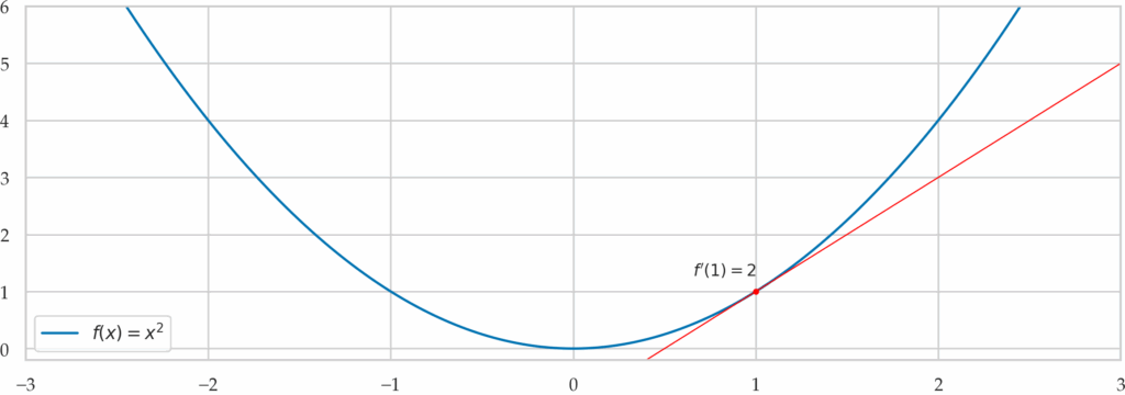
Figure 1. Illustration of the derivative of the function $f(x)= x^2$ at $x=1$. The derivative is denoted $f^{\prime\!}(1)$ and describes the slope function at the point $x=1$.

 

 

Here is the Python code for computing a numerical approximation to the derivative of the function f at the point x:

def differentiate(f, x, delta=1e-9):
    """
    Compute the derivative of the function `f` at `x`
    using a slope calculation for very short `delta`.
    """
    df = f(x+delta) - f(x)
    dx = (x + delta) - x
    return df / dx

As you can see, the code is nearly identical to the math formula. The big difference is that you can run the code! The notebook will show you examples of derivative computations using the function differentiate.

 

The integrals $\int_{a}^{b}\!f(x)\,dx$ computes the area under the graph of the function $f(x)$ between $x=a$ and $x=b$. We can compute the integral by approximating the area using $n$ rectangular strips:
\[
\int_{a}^{b}\!f(x)\,dx = \lim_{n\to\infty} \sum_{k=1}^{n} f(a + k\Delta x)\Delta x
\quad\text{where}\quad
\Delta x = \frac{b-a}{n}.
\]

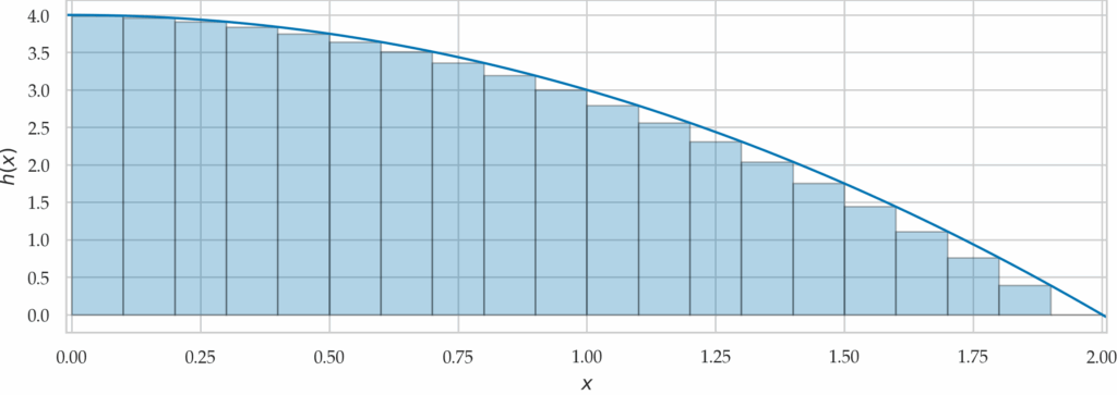
Figure 2. An approximations to the area under the graph of the function $h(x)=4-x^2$ computed using $n=20$ rectangles.  The approximation will get better and better as we increase the number of rectangles $n$.

 

We can easily turn this math formula into a Python procedure that performs the $n$-rectangle area approximation calculation.

def integrate(f, a, b, n=10000):
    """
    Computes the area under the graph of `f`
    between `x=a` and `x=b` using `n` rectangles.
    """
    dx = (b - a) / n # width of rectangular strips
    xs = [a + k*dx for k in range(1,n+1)]
    fxs = [f(x) for x in xs] # heights of the strips
    area = sum([fx*dx for fx in fxs]) # total area
    return area

We can now use this function to compute the integrals of various functions.

This helper function differentiate and integrate give us a practical, tangible computational perspective on calculus operations. However, these functions are far too slow to use for practical scientific computing tasks, which may require computing thousands or millions of derivatives and integrals.

Numerical calculations using NumPy and SciPy

The Python libraries NumPy and SciPy provide high-performance functions for doing calculus. These professional-grade functions are better suited for practical real-world calculations. The tutorial includes code examples of calculations using NumPy and SciPy, because I want you to learn about the practical methods that you’ll need outside the classroom setting.

Every computer (and even phone!) has built within it high-performance hardware specialized for doing numerical math calculations. We’re talking about processors capable of doing trillions of calculations per second! Learning a thing or two about NumPy makes all this power available to you. Newton and Leibniz could only have dreamed of the computational power that is available to us today!

 

By the end of this tutorial, you’ll have seen the core calculus concepts explained from six different perspectives: using words, graphs, math formulas, and three types of Python code (as simple Python functions written from scratch, symbolically using SymPy, and numerically using NumPy/SciPy). I hope this redundancy will help you understand the material better and learn about the real-world use cases of calculus.

 

Got feedback for me?

I hope you have a chance to print the tutorial and read it in the coming days. Please let me know if it made sense and if it helped you (re)learn calculus.

• Did the mix of math formulas and code examples work for you?
• Are there any parts that could be cut to reduce the page count?
• Are there any important topics that are missing and should be added?

You can leave comments below or email me at ivan@minireference.com as usual.