Learning statistics is greatly facilitated by using a computational platform for doing statistics calculations and visualizations. You can do basic stats calculations using pen-and-paper for small datasets, but you’ll need a computer to help you with larger datasets. Common computational platforms for doing statistics include JASP, jamovi, SPSS, R, and Python, among many others. You can even do statistics calculations using spreadsheet software like Excel, LibreOffice calc, or Google Sheets. I believe using Python is the best computational platform for learning statistics. Specifically, an interactive notebook environment like JupyterLab provides the best-in-class tools for data visualizations and probability calculations.
But what about learners who are not familiar with Python? Should we abandon non-tech learners and say they can’t learn statistics because they don’t know how to use Python? Naaaah, we ain’t having none of that! Instead, my plan is to bring non-technical learners up to speed on Python by teaching them the Python basics that they need to use for statistics. Anyone can learn Python, it’s really not a big deal. I hope to convince you of this fact in this blog post, which is intended as a Python crash-course for the absolute beginner.
I know the prospect of learning Python might seem like a daunting task, but I assure you that it is totally worth it because Python will provide you with all the tools you need to handle the mathematical and procedural complexity inherent to statistics. Using Python will make your statistics learning journey much more intuitive (because of the interactivity) and practical (because of the useful tools). All the math equations we need to describe statistical concepts will become a lot easier to understand once you can express math concepts as Python code you can “play” with. Basically, what I’m saying is that if you accept Python in your heart, you’ll benefit from much reduced suffering on your journey of learning statistics.
This blog post is the first part in a three-part series about why learning PYTHON+STATS is the most efficient and painless way to learn statistics. In this post (PART 1 of 3), we’ll introduce the JupyterLab computational platform, show basic examples of Python commands, and introduce some useful libraries for doing data visualizations (Seaborn) and data manipulations (Pandas). The key point I want to convince you of, is that you don’t need to become a programmer to benefit from all the power of the Python ecosystem, you just need to learn how to use Python as a calculator.
Table of Contents
Interactive notebook learning environments
One of the great things about learning Python is the interactivity. In an interactive coding environment, you can write some commands, run the commands, then immediately see the outputs. The immediate link between Python commands and their results makes it easy to try different inputs and make quick changes to the code based on the results you get.
A Jupyter notebook is a complete statistical computing environment that allows you to run Python code interactively, generate plots, run simulations, do probability calculations, all in the same place. All the code examples in this blog post were copy-pasted from the notebook shown in Figure 1.
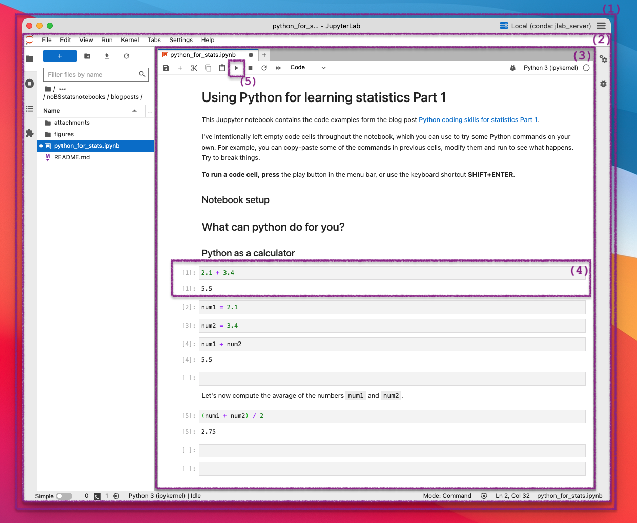
Figure 1: Screenshot of a Jupyter notebook running in JupyterLab Desktop application under macOS.
I’ve highlighted a few regions in the screenshot so that I can draw your attention to them and explain the “stack” of software that produced this screenshot. Region (1) is JupyterLab Desktop, which is an application you can download and install locally to run JupyterLab on your computer; region (2) is the JupyterLab software we use for running Jupyter notebooks; region (3) is a particular notebook called python_for_stats.ipynb (a document) that is currently opened for editing interactively; region (4) is an individual code cell that is part of the notebook.
Each cell in a notebook acts like an “input prompt” for the Python calculator. For example, the code cell (4) in the screenshot shows the input expression 2.1 + 3.4 and the output of this expression 5.5 displayed below it. This is how all code cells work in a notebook: you type in some Python commands in the code cell, then press the play button (see (5) in the screenshot) in the menu bar or use the keyboard shortcut SHIFT+ENTER, then you’ll see the result of your Python commands shown on the next line.
Running Jupyter notebooks interactively
Since Python is a popular programming language used in many domains (education, software, data science, machine learning, etc.), people have developed multiple options for running Python code. Here are some of the ways you can run the Python code in the notebook python_for_stats.ipynb interactively.
- JupyterLab: Use this link (bit.ly/py4stats1) to run the notebook python_for_stats.ipynb on a temporary JupyterLab server in the cloud. The servers are contributed by volunteer organizations (universities and web companies). This is my favorite option for running notebooks, since it doesn’t require installing anything on your computer.
- Colab: Use the colab link to run python_for_stats.ipynb in a Google Colab web environment.
- JupyterLab Desktop: Download and install the JupyterLab Desktop application on your computer. You can then right-click and choose “Save as” to save a copy of the file python_for_stats.ipynb on your computer, then open it from within the JupyterLab Desktop application. (See Figure 1).
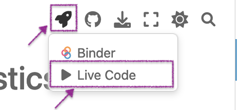 Live Code: Use the “Rocket > Live Code” menu option on the web version of the notebook.
- VS Code: Another option would be to open the file python_for_stats.ipynb in Visual Studio Code after enabling the Jupyter extension. Right-click and choose “Save as” to save a copy of the file python_for_stats.ipynb to your computer, then open it from within Visual Studio Code.
I invite you to use one of the above methods to open the notebook python_for_stats.ipynb and try running the code examples interactively while reading the rest of the blog post.
Why is interactivity important?
When learning a new skill, you’ll make a lot of mistakes. If you receive instant feedback about your actions, this makes it much easier to learn the new skill. Imagine having a private tutor looking over your shoulder, and telling you when you make mistakes. That would be nice, right?
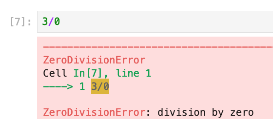
Running Python interactively in a notebook environment offers precisely this experience. Whenever you input some Python command that contains an error, Python will tell you right away by printing an “error message.” The error message tells you what problem occurred and where it occurred (highlighted in yellow). For example, if you try to divide a number by zero, Python will respond with a big red message that tells you this is not possible to do. Like, mathematically impossible. What does dividing a quantity into 0 equal parts mean? If you try 3/0 on a calculator, it will also complain and show you an error message.
Reading a Python error message gives you hints about how to fix the input so it doesn’t cause an error. In this case there is no fix—just don’t be dividing by zero! This was just a simple example I used to show what an error looks like. Yes I know the red background is very intimidating, as if chastising you for having done something wrong! Once you get used to the “panic” coloring though, you’ll start to appreciate the helpful information that is provided in these error messages. This is just your friendly Python tutor telling you something in your input needs a fix.
Receiving error messages whenever you make mistakes is one of the main reasons why learning Python is so easy. You don’t need to read a lengthy book about Python programming, you can get started by opening a Jupyter notebook and trying some commands to see what happens. The interactive feedback of notebook environments helps many people get into a learning loop that motivates them to learn more and more.
What can Python do for you?
Python is the #1 most popular language according to the TIOBE programming language popularity index. Did this happen by chance, or is there something special about Python? Why do people like Python so much? Let’s find out.
Using Python as a calculator
Python is like the best calculator ever! You can use Python for any arithmetic calculation you might want to do. Each cell in a Jupyter notebook is like the input prompt of a calculator, so if you wanted to add two numbers, you would do it like this:
 In[1]: 2.1 + 3.4
Out[1]: 5.5
All the sections in fixed-width font in this blog post contain Python code. Don’t worry if you haven’t seen code before, I’ll make sure to explain what each code block does in the surrounding text so you’ll know what’s going on. In the above code example, the first line In[1] shows the input expression we asked Python to compute, and the line Out[1] shows the output of this expression—the result that Python computed for us. This Python code example is equivalent to entering the number 2.1 on a calculator, followed by pressing the + button, then entering 3.4, and finally pressing the = button. Just like a calculator, Python computed the value of the input expression 2.1+3.4 and printed the output 5.5 on the next line.
Instead of working with numbers directly, we can store numbers into variables and specify the arithmetic operation in terms of these variables.
 In[2]: num1 = 2.1
 In[3]: num2 = 3.4
 In[4]: num1 + num2
Out[4]: 5.5
The effect of the input line In[2] is to store the number 2.1 into the new variable named num1. This is called an assignment statement in Python, and it is read from right-to-left: “store 2.1 into num1“. Assignment statements don’t have any outputs, so this is why there is no Out[2] to show. The input In[3] stores 3.4 into the variable num2, and again there is no output to display, since this is another assignment statement. The input In[4] asks Python to compute the value of the expression num1 + num2, that is, the sum of the variables num1 and num2. The result is displayed on the line Out[4].
Note the computation on line In[4] makes use of the variables num1 and num2 that were defined on the previous lines In[2] and In[3]. Python is a calculator that remembers previous commands. When Python evaluates the input line In[n], the evaluation is done in the context that includes information from all previous inputs: In[1], In[2], …, In[n-1]. This is a key paradigm you need to get used to when reading Python code. Every line of Python code runs in a “context” that includes all the commands that preceded it.
I know this sounds complicated, and you might be wondering why I’m inflicting this knowledge upon you in such an early stage of this introduction to Python. You have to trust me on this one—you need to know how to “run” a line of Python code and simulate in your head what it’s going to do. Let’s look at the input line In[4] as an example. I’ll narrate what’s going on from Python’s point of view:
I’ve been asked to evaluate the expression
num1 + num2which is the sum of two variables. The first thing I’m going to do is look up what the namenum1corresponds to in the current context and I’ll see thatnum1is a variable we defined earlier when we stored the value 2.1 into it. Similarly, I will look up the namenum2and find it has the value3.4because of the assignment statement we made on lineIn[3]. After these two lookups, I know thatnum1 + num2refers to the sum of two numbers, and I’ll compute this sum, showing the result on the output lineOut[4].
Does this make sense? Can you put yourself in Python’s shoes and see how Python interprets the commands it received and runs them?
Let’s look at another code example that shows how we can compute the average of the two numbers num1 and num2. The average of two numbers is the sum of these numbers divided by two:
 In[5]: (num1 + num2) / 2
Out[5]: 2.75
Using math notation, the average of the numbers $x_1$ and $x_2$ is expressed as $(x_1 + x_2)/2$, which is very similar. Note we used the parentheses ( and ) to tell Python to compute the sum of the numbers first, before dividing by two. I’m showing this example to illustrate the fact that the syntax of the Python expression (num1+num2)/2 is very similar to standard math notation $(x_1 + x_2)/2$. If you know the math notation for plus, minus, times, divide, exponent, parentheses, etc. then you already know how the Python operators +, -, *, /, ** (exponent),( and ) work.
Remember that the best way to learn Python is to “play” with Python interactively. If you’re a Python beginner, I highly recommend you follow along all the examples in this blog post in an interactive prompt where you can type in commands and see what comes out. Remember, you can run this notebook by clicking on the JupyterLab binder link, the colab link, or by enabling the Live Code feature from the rocket menu on the web version.
In order to make it easy for you to copy-paste code blocks from this blog post into a notebook environment, from now on, I won’t show the input indicators In[n]: and instead show only the input commands. This will allow you to copy-paste commands directly into a Python prompt (Live Code webpage or notebook) and run them for yourself to see what happens. Here is a repeat of the input-output code from the previous code block using the new format.
(num1 + num2) / 2
# 2.75
The input on the first line is the same as the input line In[5] we saw above. The second line shows the output prefixed with the #-character (a.k.a. hash-sign), which is used to denote comments in Python. This means the line # 2.75 will be ignored by the Python input parser. The text # 2.75 is only there for reference—it tells human readers what the expected output is supposed to be. Try copy-pasting these lines into a code cell inside your choice of a Python interactive coding environment. Run the code cell to check that you get the expected output 2.75 as indicated in the comment.
Powerful primitives and builtin functions
Python is a “high level” programming language, which means it provides convenient data structures and functions for many common calculations. For example, suppose you want to compute the average grade from a list that contains the grades of the students in a class. We’ll assume the class has just four students, to keep things simple.
The math expression for computing the average grade for the list of grades $[g_1,g_2,g_3,g_4]$ is $(g_1 + g_2 + g_3 + g_4) / 4 = (\sum_{i=1}^{i=4} g_i ) / 4$. The symbol $\Sigma$ is the greek letter Sigma, which we use to denote summations. The expression $\sum_{i=1}^{i=4} g_i$ corresponds to the sum of the variables $g_i$ between $i=1$ and $i=4$. This is just fancy math notation for describing the sum $g_1 + g_2 + g_3 + g_4$.
The code example below defines the list grades that contains four numbers, then uses the Python builtin functions sum and len (length) to compute the average of these numbers (the average grade for this group of four students).
grades = [80, 90, 70, 60]
avg = sum(grades) / len(grades)
avg
# 75.0
The first line of the above code block defines a list of four numbers [80,90,70,60] and stores this list of values in the variable named grades. The second line is an assignment statement, where the right hand side computes the sum of the grades divided by the length of the list, which is the formula for computing the average. The result of the sum-divided-by-length calculation is stored into a new variable called avg (short for average). Finally, the third line prints the contents of the variable avg to the screen.
Dear readers, I know all of the descriptions may feel like too much information (TMI), but I assure you learning how to use Python as a calculator is totally worth it. It’s really not that bad, and you’re already ahead in the game. If you were able to follow what’s going on in the above code examples, then you already know one of the most complicated parts of Python syntax: the assignment statement.
Python reading exercise: revisit all the lines of code above where the symbol = appears, and read them out loud, remembering you must read them from right-to-left: “compute <right hand side> then store the result into <left hand side>”. That’s what the assignment statement does: it evaluates some expression (whatever appears to the right of the =) and stores the result into the place described by the left-hand side (usually a variable name).
There are two more Python concepts I would like to introduce you to: for-loops and functions. After that we’re done, I promise!
For loops
The for-loop is a programming concept that allows us to repeat some operation or calculation multiple times. The most common use case of a for-loop is to perform some calculation for each element in a list. For example, we can use a for loop to compute the average of the numbers in the list grades = [80,90,70,60]. Normally, we would compute the average using the expression avg = sum(grades)/len(grades), but suppose we don’t have access to the function sum for some reason, and so we must compute the sum using a for-loop.
We want to compute the sum 80 + 90 + 70 + 60, which we can also write as 0 + 80 + 90 + 70 + 60, since starting with 0 doesn’t change anything. We can break up this summation into a four-step process, where we add the individual numbers one by one to a running total, as illustrated in Figure 2.

Figure 2: Step-by-step calculation of the sum of four numbers. In each step we add one new number to the current total. This procedure takes four steps: one step for each number in the list.
Note the operation we perform in each step is the same—we add the current grade to the partial sum of the grades from the previous step.
Here is the Python code that computes the average of the grades in the list grades using a for-loop:
total = 0
for grade in grades:
    total = total + grade
avg = total / len(grades)
avg
# 75.0
The first line defines the variable named total (initially containing 0), which we’ll use to store the intermediate values of the sum at different steps. Next, the for loop tells Python to go through the list grades and for each grade in the list, perform the command total = total + grade. Note this statement is indented relative to the other code to indicate it is “inside” the for loop, which means it will be repeated for each element in the list. On the next line we divide the total by the length of the list to obtain the average, which we then display on the fifth line.
A for-loop describes a certain action or actions that you want Python to repeat. In this case, we have a list of grades $[g_1, g_2, g_3, g_4]$, and we want Python to repeat the action “add $g_i$ to the current total” four times, once for each number $g_i$ in the list. The variable total takes on different values while the code runs. Before the start of the for-loop, the variable total contains 0, we’ll refer to this as total0. Then Python starts the for-loop and runs the code block total = total + grade four times, once for each grade in the list grades, which has the effect of changing the value stored in the variable total four times. We’ll refer to the different values of the variable total as total1, total2, total3, and total4. See Figure 3 for the intermediate values of the variable total during the four steps of the for loop.

Figure 3: Mathematical description and computational description of the procedure for computing the average in four steps. The label totalk describes the value stored in the variable total after the code inside the for loop has run k times.
The key new idea here is that the same line of code total = total + grade corresponds to four different calculations. Visit this page to see a demonstration of how the variable total changes during the four steps of the for loop. At the end of the for loop, the variable total contains 300 which is the sum of the grades, and calculating total/len(grades) gives us the average grade, which gives the same result as the expression sum(grades)/len(grades) that we used earlier.
If this is the first time you’re seeing a for-loop in your life, the syntax might look a little weird, but don’t worry you’ll get used to it. I want you to know about for-loops because we can use for-loops to generate random samples and gain hands-on experience with statistics concepts like sampling distributions, confidence intervals, and hypothesis testing. We’ll talk about these in PART 2 of the series.
Functions
Python is a useful calculator because of the numerous functions it comes with, which are like different calculator buttons you can press to perform computations.
We’ve already seen the function sum that computes the sum of a list of elements. This is one of the builtin Python functions that are available for you to use. You can think of sum as a calculator button that works on lists of numbers. Readers who are familiar with spreadsheet software might have already seen the spreadsheet function SUM(<RANGE\>) which computes the sum for a <RANGE\> of cells in the spreadsheet.
Here are some other examples of Python built-in functions:
len: computes the length of a listrange(0,n): creates a list of numbers[0,1,2,3, ..., n-1]min/max: finds the smallest/largest value in a listprint: prints some value to the screenhelp: shows helpful documentation
Learning Python is all about getting to know the functions that are available to you.
Python also makes it easy to define new functions, which is like adding “custom” buttons to the calculator. For example, suppose we want to define a new button mean for computing the mean (average) of a list of values. Recall the math notation for calculating the average value for the list $[x_1, x_2, x_3, \ldots, x_n]$ is $(\sum_{i=1}^{i=n} x_i)/n$.
To define a Python function mean we can use the following code:
def mean(values):
    total = 0
    for value in values:
        total = total + value
    avg = total / len(values)
    return avg
Let’s go through this code example line by line. To define a new Python function, we start with the keyword def followed by the function’s name, we then specify what variables the function expects as input in parentheses. In this case the function mean takes a single input called values. We end the line with the symbol :, which tells us the “body” of the function is about to start. The function body is an indented code block that specifies all the calculations that the function is supposed to perform. The last line in the function body is a return statement that tells us the output of the function. Note we’ve seen the calculations in the body of the function previously, when we computed the average of the list of grades grades = [80,90,70,60] using a for-loop.
The function mean encapsulates the steps of the procedure for calculating the mean and makes it available to us as a “button” we can press whenever we need to compute the mean of some list of numbers.
To call a Python function, we write its name followed by the input argument specified in parentheses. To call the function mean on the list of values grades, we use the following code:
mean(grades)
# 75.0
When Python sees the expression mean(grades) it recognizes it as a function call. It then looks for the definition of the function mean and finds the def statement we showed in the previous code block, which tells us what steps need to be performed on the input.
The function mean can compute the average for any list of values, but when we call mean(grades) we are supplying the specific list grades as the input values. In other words, calling a function mean with the input grades is equivalent to the assignment statement values = grades, then running the code instructions in the body of the function. The return statement on the last line of the function’s body tells us the function output value is avg. After the function call is done, the expression mean(grades) gets replaced with the return value of the function, which is the number 75. Click here to see the visualization of how this code runs.
Calling a function is like delegating some work to a contractor. You want to know the mean of the numbers in the list grades, so you give this task to the function mean, which does the calculation for you, and returns to you the final value.
Okay that’s it! If you were able to understand the Python code examples above, then you already know the three Python syntax primitives that you need for 90% of statistics calculations. If you want to learn more about Python, take a look at the Python tutorial (Appendix C), which is a beginner-friendly introduction to Python syntax, data types, and builtin functions.
But wait there’s more…. I haven’t even shown you the best parts yet!
A rich ecosystem of Python libraries
Python is a popular language because of the numerous functions it comes with. You can “import” various Python modules and functions to do specialized calculations like numerical computing (NumPy), scientific computing (SciPy), data management (Pandas), data visualization (Seaborn), and statistical modelling (statsmodels).
We’ll now briefly mention a few of the Python libraries that are useful when learning statistics:
- Pandas is the Swiss army knife of data manipulations. Pandas provides functions for loading data from various formats (CSV files, spreadsheets, databases, etc.). Once you have loaded your data, Pandas provides all the functions you might need for data processing, data cleaning, and descriptive statistics. See below for basic code examples. Check the tutorial and the docs for more info.
- Seaborn allows you to generate beautiful data visualizations. When working with data, we often want to generate statistical visualizations like strip plots, scatter plots, histograms, bar plots, box plots, etc. The library Seaborn offers functionality for creating such plots and all kinds of other data visualizations. Check out the gallery of plot examples to get an idea for the types of plots you can generate using Seaborn. See below for basic examples or check the tutorial and the docs for more details.
- NumPy and SciPy contain all the scientific computing functions you might need. In particular, the module
scipy.statscontains all the probability models we use in statistics. We’ll show some examples of probability models in PART 2. - Statsmodels is a statistical modelling library that includes advanced statistical models and pre-defined functions for performing statistical tests.
- SymPy is a library for symbolic math calculations. Using SymPy you can work with math expressions just like when solving math problems using pen and paper. SymPy calculations are useful because functions like
solve,simplify,expand, andfactorcan do the math for you. See the tutorial for more info and try some commands in the SymPy live shell.
So yes, Python is just like a calculator, but because it comes with all the above libraries, it’s like the best calculator ever! We’ll now show some examples that highlight the usefulness of the Seaborn library for data visualizations.
Data visualization using Seaborn
The first part of any statistical analysis is to look at the data. Descriptive statistics is a general term we use to refer to all the visualizations and calculations we do based on a sample in order to describe its properties. Statistical plots give us visual summaries for data samples. Examples of such plots include scatter plots, bar plots, box plots, etc. We can easily create all these visual summaries using the Python library Seaborn, which makes statistical plotting very straightforward.
Let’s look at some examples of data visualizations based on a sample of prices, which we will represent as a list of nine values (prices collected at different locations).
prices = [11.8, 10, 11, 8.6, 8.3, 9.4, 8, 6.8, 8.5]
Next we’ll import the module seaborn under the alias sns.
import seaborn as sns
This is called an “import statement” in Python, and its effect is to make all the functions in the seaborn module available by calling them as sns.<functionname\>. We use the alias sns instead of the full module name seaborn to save a few keystrokes.
Statistical plots can be generated by specifying prices as the x-input to one of the seaborn plot-functions. We can use sns.stripplot to generate a strip plot, sns.histplot to generate a histogram, or sns.boxplot to generate a box-plot, as shown below:
sns.stripplot(x=prices, jitter=0)
# See Figure 4 (a)

sns.histplot(x=prices)
# See Figure 4 (b)

sns.boxplot(x=prices)
# See Figure 4 (c)
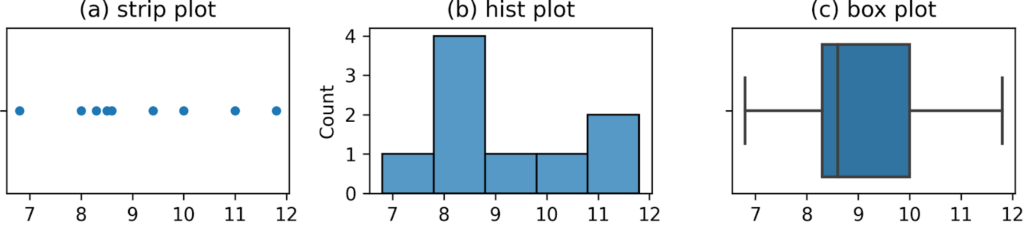
Figure 4. Three common types of statistics visualizations.
The plot shown in Figure 4 (a) shows the “raw data,” with each value in the prices list represented as a separate point, whose $x$-location within the graph corresponds to the price. The histogram in Figure 4 (b) shows what happens when we count the numbers of observations in separate “bins.” The higher the bar, the more observations in that bin. Finally, the box-plot in Figure 4 (c) shows the location of the quartiles of the prices data (to be defined shortly).
Data visualization is an essential part of any statistical analysis, and the Seaborn library is a best-in-class tool for doing statistical visualizations: box plots, histograms, scatter plots, violinplots, etc. Anything you might want to do, there is probably a plot function for it in Seaborn. As a first step to learning Seaborn, you can check out the Seaborn tutorial (Appendix E), which explains the essential Seaborn plotting functions that we use in the book.
Data manipulations with Pandas
Data is the fuel for statistics. All statistical calculations start with data collection and processing. The Python library Pandas provides lots of helpful functions for data manipulations. Understanding what Pandas can do is best done through examples, so we’ll now show some real-world code examples of using Pandas. We don’t have time to explain all the details, so we’ll use the show-don’t-tell approach in this section.
Electricity prices dataset
We’ll use a dataset epriceswide.csv which consists of 18 samples of electricity prices collected from charging stations in the East End and the West End of a city. Figure 5 shows the data as appears when viewed online, when opened with a simple text editor, and when viewed using spreadsheet software like LibreOffice Calc.
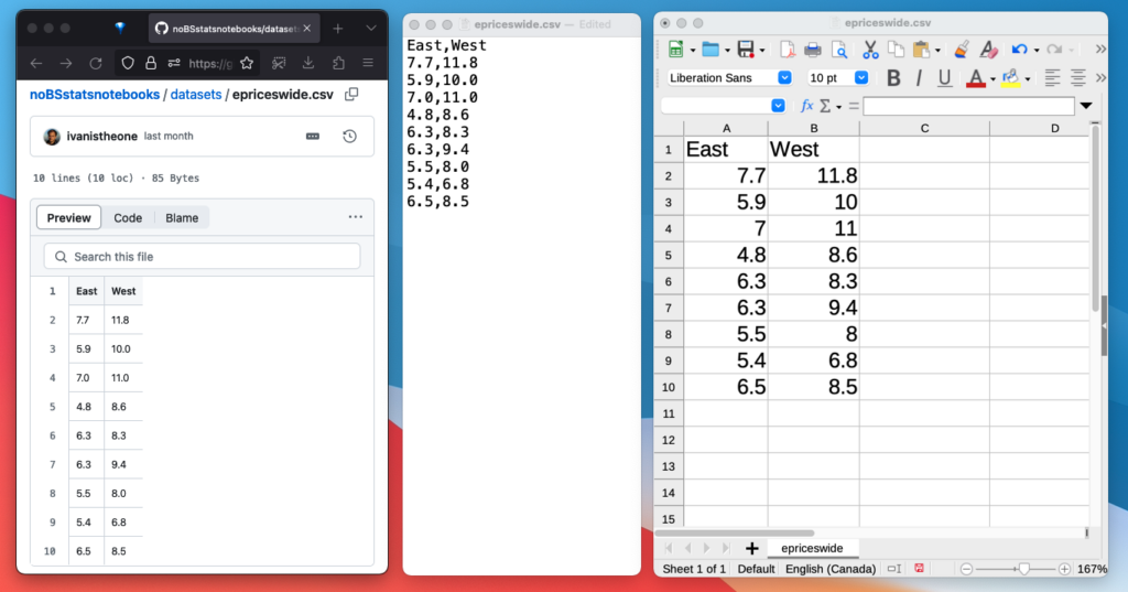
Figure 5: The dataset epriceswide.csv viewed online, in a text editor, and in spreadsheet software.
We call this data format CSV, which is short for comma-separated values. CSV files are very common in both industry and academia, since they are a very simple data format that can be opened with many software tools.
Data extraction
We can use the function read_csv from the Pandas module to load the data from a CSV file, which can be a local file or a URL (an internet location). Pandas provides other functions like read_excel and read_db_table for loading data from other data formats.
Let’s look at the commands we need to load the data file epriceswide.csv from a web URL .
import pandas as pd
epriceswide = pd.read_csv("https://nobsstats.com/datasets/raw/epriceswide.csv")
epriceswide
#    East  West
# 0   7.7  11.8
# 1   5.9  10.0
# 2   7.0  11.0
# 3   4.8   8.6
# 4   6.3   8.3
# 5   6.3   9.4
# 6   5.5   8.0
# 7   5.4   6.8
# 8   6.5   8.5
The first line import pandas as pd imported the pandas library under the alias pd. This is similar to how we imported seaborn as sns. The shorter alias will save us some typing. Next we call the function pd.read_csv to load the data, and store the result in a variable called epriceswide, which we then print on the next line. The variable epriceswide contains a Pandas data frame, which is similar to a spreadsheet (a table of values whose rows are numbered and whose columns have names).
The data frame epriceswide contains two columns of prices from the West End and the East End of a city.
I’m interested only in the prices in the West End of the city (the second column). To extract the prices from the West End of the city we use the following Pandas code.
pricesW = epriceswide["West"]
pricesW
# 0    11.8
# 1    10.0
# 2    11.0
# 3     8.6
# 4     8.3
# 5     9.4
# 6     8.0
# 7     6.8
# 8     8.5
The square brackets syntax has the effect of selecting the data from one of the columns. The variable pricesW corresponds to a Pandas series object, which is similar to a list, but has many useful functions “attached” to it.
Descriptive statistics using Pandas
We can easily compute summary statistics like the mean, the median, the variance, the standard deviation, etc., from any Pandas data frame or series by calling a function of the same name: mean, median, var, std, etc. These numerical summaries are called descriptive statistics, and they are very useful for understanding the characteristics of the dataset.
For example, to see the number of observations in the series pricesW(the sample size), we use the function .count().
pricesW.count()
# 9
Note the syntax is pricesW.count() and not count(pricesW). This is because the function count() is “attached” to the pricesW object. Functions attached to objects are called methods. The syntax for calling a method is a little weird, obj.fun(), but the effect is the same as fun(obj).
To compute the sample mean $\overline{\mathbf{x}} = \frac{1}{n} \sum_{i=1}^9 x_i$, we call the .mean() method on pricesW.
pricesW.mean()
# 9.155555555555557
To compute the median (50th percentile), we call the .median() method:
pricesW.median()
# 8.6
To compute the sample standard deviation $s_{\mathbf{x}} = \sqrt{ \frac{1}{n-1}\sum\nolimits_{i=1}^n \left(x_i – \overline{\mathbf{x}} \right)^2 }$, we call the .std() method:
pricesW.std()
# 1.5621388471508475
Note the standard deviation is a complicated math formula involving subtraction, squaring, summation, divisions, and square root, but we didn’t have to do any of these math operations, since the predefined Pandas function std did the standard deviation calculation for us. Thanks Pandas!
The method .describe() computes all numerical descriptive statistics for the sample in one shot:
pricesW.describe()
# count     9.000000
# mean      9.155556
# std       1.562139
# min       6.800000
# 25%       8.300000
# 50%       8.600000
# 75%      10.000000
# max      11.800000
This result includes the count, the mean, the standard deviation, as well as a “five-number summary” of the data, which consists of the minimum value (0th percentile), the first quartile (25th percentile), the median (50th percentile), the third quartile (75th percentile), and the maximum value (100th percentile).
Data cleaning using Pandas
Another important class of transformations is data cleaning: making sure data values are expressed in a standardized format, correcting input errors, and otherwise restructuring the data to make it suitable for analysis. Using various filtering and selection functions within Pandas allows you to do most data cleaning operations without too much trouble.
Using Pandas for data loading, data transformations, and data cleaning are useful skills to develop if you want to apply statistics to real-world situations. To learn more about Pandas, I’ll refer you to the notebook for Section 1.3 which is a condensed crash course on Pandas methods for descriptive statistics, and the Pandas tutorial (Appendix D) which contains info about data manipulation techniques.
How much Python do you need to know?
After all this talk about learning Python, I want to remind you that you don’t need to become a Python programmer! As long as you know how to use Python as a calculator, then you’re in business. Specifically, here are the skills I believe everyone can pick up:
- run code cells in an interactive notebook environment (using JupyterLab online or on your computer)
- know how to open/edit notebooks (I’ve prepared notebooks to accompany each section in the book)
- run data visualization code examples (i.e. use basic Seaborn functions)
- run code examples for data manipulations (i.e. use Pandas for loading datasets)
- experiment by changing parameters in existing simulations
Even if you’re an absolute beginner in Python and don’t want to learn Python, you can still benefit from the code examples in the notebooks as a spectator. Just running the code and seeing what happens. You’ll also be able to solve some of the exercises by simply copy-pasting commands.
Once you gain some experience with basic Python commands and learn the common function of the Pandas and Seaborn libraries, you’ll be able to apply these skills to load new datasets and generate your own visualizations. Learning Pandas and Seaborn will allow you to tackle real world datasets, not just the ones prepared for this book.
Your knowledge of basic Python will be very helpful for understanding probability and statistics. Here are some examples of activities that will be available to you:
- use the
scipy.statsprobability models (these are the LEGOs of the XXIst century) - run probability simulations
- perform statistical analyses (multi-step procedures with lots of complicated steps)
- use Python calculations to verify statistical results like p-values and confidence interval coverage probabilities
We’ll talk more about these in PART 2 of the blog post series.
I want to emphasize that all these calculations are accessible in “spectator mode” where you run the notebooks to see what happens, without any expectation of writing new code. As you gain more Python experience over time, you’ll be able to modify the code examples and adapt them to solving new problems.
Conclusion
I hope the code examples in this blog post convinced you that learning Python is not that complicated. I also hope you take my word for it that knowing how to use Python as a calculator will be very helpful when learning statistics.
In the next post (PART 2 of 3) we’ll talk about specific probability and statistics concepts that become easier to understand when you can “play” with them using the Python calculator. Indeed, Python makes working with fancy, complicated, mathy topics like random variables and their probability distributions as easy as playing with LEGOs. We can also use Python to run probability simulations, which can be very helpful for understanding conceptually-difficult concepts like sampling distributions.
In the final post (PART 3 of 3) I’ll describe how the PYTHON+STATS curriculum is packaged and delivered in the upcoming textbook No Bullshit Guide to Statistics. I’ve been working on this book for the past 5+ years, continuously optimizing the structure of the book to make it accessible for the average reader. I want every adult learner who wants to learn statistics to have a concise guide to the material, including explanations for how things work “under the hood” in terms of probability calculations.
Links for further reading
Here are some suggestions for further reading:
- Read the Python tutorial which contains a concise introduction to Python for absolute beginners.
- Check out the links in the Pandas tutorial and the Seaborn tutorial to learn more about these libraries.
- To learn more about the No Bullshit Guide to Statistics, visit the detailed outline gdoc, the concept map pdf, or visit the book’s website noBSstats.com, which contains all the notebooks from the book. Sign up here to receive progress updates about the book and get notified when it is ready for purchase.
- I’m also looking for test readers to provide feedback on draft chapters. Sign up here to become a test reader and I’ll send you PDF previews of chapter/section drafts once every few weeks. As a test reader, I expect you to dedicate a few hours to reading the drafts and send me feedback by email, e.g. to highlight when some explanations are confusing.
- See the Links to STATS 101 Learning Resources gdoc for a lot more links to the best statistics tutorials, books, courses, video lectures, and websites.
PS: Why not R?
This question is bound to come up, so I’ll go ahead and answer it preemptively. The R ecosystem (R, RStudio, RMarkdown, Quarto, CRAN packages, tidyverse, etc.) is also a very good platform for learning statistics. Some might even say R is better than Python, since it is a programming language specially designed for statistics. Certainly, if your goal is to learn advanced statistical techniques, then learning R would be a good choice given the numerous packages available in R. For learning basic statistics, however, R and Python are equally good.
I chose Python for the book because it is an easy language to learn, with minimal syntax rules, and good naming conventions. Python is a general purpose language, which means the Python skills you develop for statistical calculations can be used for all kinds of other tasks beyond statistics including, web programming, data science, and machine learning. Learning Python will make you part of a community of millions of Pythonistas (people who use Python), which makes it very likely you’ll be able to find help whenever you get stuck on a problem, and find lots of learning resources for beginners.
All this being said, I still think R is very useful to know, and I plan to release R notebooks to accompany the book at some point. A multi-language approach would be great for learning, since you see the same concept explained twice, which is good for understanding the underlying statistical principles.
DIOGO PEDROZA LOUREIRO
November 12, 2024 — 12:08 pm
I can’t wait for your statistics book. When is it going to be released?
ivan
November 12, 2024 — 1:27 pm
It’s coming soon. I’m now writing the last chapter, but I have already gone thought edits on the first few chapters. I’m hoping for initial release in early January 2025.